
Building a Transformer LLM with Code: Evolution of Positional Encoding
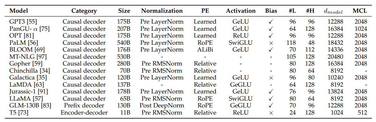
In our previous blog, we delved into the implementation and training of a GPT-based transformer model, incorporating several minor optimizations. The transformer architecture has showcased remarkable resilience to evolving trends. Beyond the PreNorm technique, another critical area that researchers have significantly improved is positional encoding. Positional encoding enables the model to comprehend the relative positions of words within a sentence, a vital factor for tasks like language translation and text generation.
The introduction of new positional embedding methods has empowered models to effectively capture larger contextual information. It has also served as a foundational element in various Language Model (LLM) architectures, including T5, Llama, and MPT.
In this post, we'll delve into the evolution of positional encoding techniques and their integration into transformer models. The final section offers a summary and comparison of these methods. You can practice these concepts by following the linked Colab Notebook, featuring step-by-step code implementation.
Hands-on Notebook: github
Experiment Dashboard: wandb
Vanilla Transformer Model
The vanilla transformer model, introduced by Vaswani et al. in 2017, uses a sinusoidal function to encode the position of each word in the input sequence. This positional encoding is added to the word embeddings before being fed into the model. The sinusoidal function has the advantage of being able to represent an arbitrary length sequence, but it has some limitations in terms of expressiveness. Authors also experimented with using learned positional embeddings but found no significant impact. So sinusoidal-based positional encoding was selected.
Integrated Positional Embedding
In later studies, it was discovered that learned positional embedding had no advantage because positional embeddings were just added initially. In deep multilayered networks, positional embedding goes through so much transformation that positional information is rendered ineffective. To improve the expressiveness of positional information in the entire network, positional information is integrated into each transformer block in the model. This involves learning a separate embedding for each position in the input sequence, for every transformer block. Integrated positional embedding has been shown to improve performance, but it has the disadvantage of requiring a fixed maximum sequence length.
We can incorporate absolute position into embedding space as:
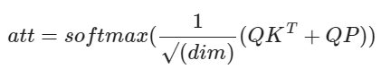
where P is the position embedding vector. This can be incorporated in MHSA implementation as follows:
class MultiHeadAttention(nn.Module):

    def __init__(self, num_heads, head_size, shared_head=False):
        super().__init__()
        self.num_heads = num_heads
        self.head_size = head_size
        self.shared_head = shared_head

        self.key = nn.Linear(head_size, head_size, bias=False)
        self.query = nn.Linear(head_size, head_size, bias=False)
        self.value = nn.Linear(head_size, head_size, bias=False)
        self.register_buffer('tril', torch.tril(torch.ones(block_size, block_size)))

        if self.shared_head:
          self.pos_emb = nn.Parameter(torch.randn(block_size, head_size))
        else:
          self.pos_emb = nn.Parameter(torch.randn(num_heads, block_size, head_size))

        self.dropout_wei = nn.Dropout(dropout)
        n_embd= num_heads*head_size
        self.proj = nn.Linear(n_embd, n_embd)
        self.dropout_proj = nn.Dropout(dropout)


    def forward(self, x):
        # Reshape the tensor to B N T H for N heads
        B,T,C = x.shape
        x = rearrange(x, 'B T (N H) -> B N T H', N=self.num_heads)

        k = self.key(x)   # (B,N,T,H)
        q = self.query(x) # (B,N,T,H)

        # compute attention scores
        q = q * self.head_size**-0.5
        wei = torch.einsum("BNTH, BNSH -> BNTS", q,k)

        # Position Embedding
        if self.shared_head:
          p_wei = torch.einsum("BNTH, SH-> BNTS" ,q,self.pos_emb[:T])
        else:
          p_wei = torch.einsum("BNTH, NSH-> BNTS" ,q,self.pos_emb[:,:T,:])

        wei += p_wei

        # final attention and value computation
        wei = wei.masked_fill(self.tril[:T, :T] == 0, float('-inf'))
        wei = F.softmax(wei, dim=-1)
        wei = self.dropout_wei(wei)
        # perform the weighted aggregation of the values
        v = self.value(x) # (B,N,T,H)
        out = torch.einsum("BNTS, BNSH -> BNTH", wei, v)

        # concat and mix N Heads
        out = rearrange(out, 'B N T H -> B T (N H)')
        out = self.dropout_proj(self.proj(out))
        return out
Another approach is to add absolute embedding to embedding x just before transforming it into K, Q, and V vectors.
Relative Position Embeddings
One limitation of absolute positional encoding lies in its lack of translation invariance. When the same sentence or phrase is shifted, the absolute positions change, resulting in different attention patterns. For instance, in the diagram below, the verb "cook" at position 1 should ideally pay higher attention to the word "She" with absolute position 0, while the same verb "cook" at position 6 should prioritize the word "I" with absolute position 5.

Relative position embeddings offer a solution to this challenge by introducing translation invariance to positional information. With relative positioning, the verb "cook" needs to consider the -1 position for the subject in both instances. This incorporation of relative position embeddings introduces an inductive bias of translation invariance into the generalized transformer architecture.This has demonstrated performance improvements in both natural language processing (NLP) and computer vision tasks.
Drawing from Shaw et al.'s 2018 proposal, we can incorporate their approach as follows:
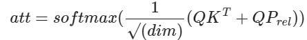
Here, 'P' represents learnable position embeddings, which enable the learning of unique representations for each relative pair of positions. This implementation has been detailed in the corresponding section in Colab.
It's worth noting a clever technique we employ in relative position embedding. Attention sequence for N token have the following relative position pattern, where 0 is current position, 1 represents next token and -1 represents previous token.

To capture all relative positions in a sequence of 'N' tokens, we require '2N-1' unique positions. In our implementation, we create a learnable embedding size of '2N-1' vectors, then employ a relative_to_absolute function to map this to the required 'NxN' pattern. This mapping is achieved through a clever combination of padding and reshaping of matrices, ensuring efficiency in computation. We take reference from Lucidrains for a non-causal implementation that enables capabilities like prefix decoders, causal decoders, and vision transformers.
For a causal-only decoder, where we don't need to attend to future tokens (positions '1', '2', '3', and so on), we only require 'N' unique relative positions, ranging from '-N+1' to '0'. There exist more optimized transformations, as proposed by Shaw et al (2018) and further refined by Huang et al (2018), for this specific scenario.
You can also find additional insights in the 'Extra' section at the end of the Colab section, which provides a step-by-step representation of how this transformation works.
Relative Bias (T5)
The T5 model, introduced by Raffel et al. in 2020, employs a technique known as "relative bias." Instead of using an embedding vector for each relative position, it utilizes a learnable scalar bias. This relative bias term is added to the corresponding logit during the computation of attention weights. This approach reduces the number of learned positional parameters, resulting in improved efficiency in terms of both memory and computation.
Mathematically, it can be expressed as:
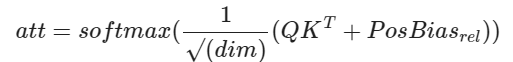
To further enhance efficiency, T5 shares the position embedding parameters across all layers in the model. However, within a given layer, each attention head utilizes a distinct learned position embedding. In our implementation, we employ relative bias for each unique relative position. It's important to note that the original T5 implementation used position binning, based on linear and logarithmic relative distances, to scale to larger contextual contexts.
Rotary Position Embedding (RoPE)
RoPE, introduced in RoFormer 2021, serves as the cornerstone of the LLama architecture and has found widespread adoption in other cutting-edge transformer models such as PaLM and Dolly. It revolutionizes the encoding of positional information for tokens by employing a rotation matrix. This matrix seamlessly incorporates explicit relative position dependencies into attention calculations. The RoPE rotation matrix offers remarkable flexibility, accommodating varying sequence lengths, diminishing inter-token dependencies as relative distances increase, and, notably, enhancing linear self-attention with relative position encoding.
The application of RoPE to Query (Q) and Key (K) vectors is elegantly simple. When you compute attention using the standard approach, it inherently infuses the result with relative position information:
q, k = self.rotary_emb.rotate_queries_and_keys(q, k)
# compute attention scores - Flash attention
out = torch.nn.functional.scaled_dot_product_attention(q, k, v, is_causal=True)
For a comprehensive understanding of its implementation, you can refer to the Colab section. For further exploration and insights, the eleutherAI Blog is an excellent resource. Additionally, you can access the official RoPE library and LLAMA Code Implementation.
One of the significant advantages of RoPE lies in addressing a key limitation of Relative Bias. Calculating relative positional bias, as done in T5, necessitates constructing a complete attention matrix for all pairs of positions in the input sequence. This operation has a quadratic time complexity, which is manageable for smaller input sequences but quickly becomes computationally intensive for longer ones. In this regard, RoPE shines, particularly when using efficient alternatives to softmax attention, including kernelized variants like FAVOR+, which don't require the computation of the full attention matrix.
Align and Bias (AliBi)

AliBi employs scalar bias values, similar to the Relative Bias technique. However, instead of learning these values, it derives them using a straightforward formula. The essence of AliBi lies in penalizing the attention assigned by a query to a key based on their relative distance. When a query and key are in close proximity, the penalty is minimal, but it significantly increases as they move farther apart.The biases decrease linearly in the log scale, and each head has a different slope. The slope calculation is as follows:
def get_slopes(n_heads: int):
    n = 2 ** math.floor(math.log2(n_heads))
    m_0 = 2.0 ** (-8.0 / n)
    m = torch.pow(m_0, torch.arange(1, 1 + n))
    if n < n_heads:
        m_hat_0 = 2.0 ** (-4.0 / n)
        m_hat = torch.pow(m_hat_0, torch.arange(1, 1 + 2 * (n_heads - n), 2))
        m = torch.cat([m, m_hat])

    return m
AliBi is very fast and is used in MPT. It was the first architecture to enable 100K context length. It outperforms Rotary embeddings in accuracy when evaluating sequences that are longer than the ones the model was trained on (extrapolation).
Landmark Attention

This is a recent attention mechanism emerging from Chinese AI research labs and has yet to be integrated into large foundational Language Model (LLM) architectures. Notably, it brings significant advancements to the attention mechanism, particularly when dealing with longer contextual information. AliBi and RoPE penalisation increases with relative position which heavily discourages the model to pick context information from large relative distance. Landmark-based approach solves this limitation. It employs a landmark token to represent the overall context of a block of text. It then leverages this landmark token to penalize the individual token attention. This innovative approach allows for efficient contribution of information from distant parts of a text block to the attention value.
I am curious to see its adoption in new LLMs. As this is more effective on longer context length, I have skipped the implementation here.
Evaluation and Comparison
Expanding upon our previous tutorial on Large Language Models (LLMs), we perform evaluations using the same tiny Shakespeare dataset. For educational purposes, I've created scaled-down versions of LLMs featuring 8 heads, 64 embedding dimensions, and a 32-token context. You're encouraged to give it a try; the training process requires only 10 minutes on Google Colab GPU. The figure below provides a comparative analysis of training parameters, as well as training and validation loss/perplexity performance.

As evident, AliBi boasts the fewest parameters, closely followed by RoPE. While the differences may appear relatively small in this context, they become more pronounced as you increase the context length from 32 tokens to 32,000 tokens or more. In our approach, Relative Bias, AliBi, and RoPE, all exhibit similar learning capabilities when considering the validation set perplexity. Importantly, this performance enhancement is achieved with the addition of only a minimal number of parameters. For a more detailed comparison, you can refer to the WandB experiment tracking dashboard.
What’s Next?
In this single post, we have successfully implemented scaled-down versions of T5 (decoder only), LLama, and MPT models from an architectural standpoint. To maintain simplicity for educational purposes, we've avoided some of the more complex optimizations. Still, it is powerful enough to showcase the effectiveness of recent relative position embedding evolution and where it is headed.
Next, we will take a look at several advancements that have been made in Efficient attention mechanisms such as Sparse Attention(BIG BIRD), FAVOR+ (Performer), MultiQuery Attention, and Longformer(Sliding Attention).