Building a Transformer LLM with Code: Fundamental Transformer & GPT
In this post, we will code fundamental Transformer blocks, and embark on a journey to build a GPT model from the ground up. Our journey starts with Karpathy's guide on GPT from scratch - implementing tokenisation, self-attention, multi-head and causal attention, and trainable transformers. Building upon this foundation, we will further improve by introducing optimisation techniques like PreNorm, weight tying, flash attention, and merged QKV computation.
While this post introduces you to essential concepts with bits of code, you can seamlessly put these concepts into practice by following along with the linked Colab Notebook, which provides a step-by-step code implementation.
Hands-on Notebook: Github
Coding Transformer: The Fundamental Block
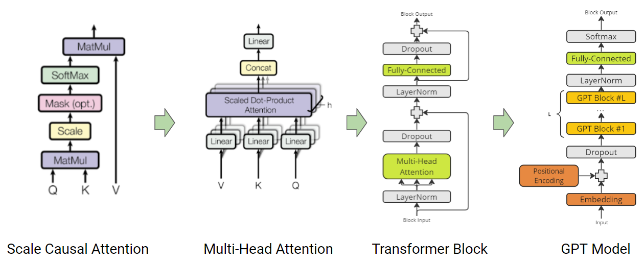
As introduced in the attention paper, Query (Q), Key (K) and Value (V) based efficient attention mechanism forms the core of the Transformer architecture. The attention mechanism calculates the output as a weighted sum of the values, where the weight assigned to each value is determined by the scaled dot-product of the query with all the keys. This allows the model to weigh the importance of each input token when making predictions.

Here’s an example of how attention can be implemented:
B, T, head_size = 4, 8, 64  # batch, token_context_length, head_size
k = torch.randn(B, T, head_size)
q = torch.randn(B, T, head_size)
v = torch.randn(B, T, head_size)

# Attention calculation
attention = torch.einsum('b t h, b s h-> b t s', q, k) * head_size ** -0.5
In Self-Attention, Q, K, and V are derived from a single input representation. On the other hand, in the domain of cross-attention, Q originates from one input, whereas K and V are extracted from another.
Casual-Attention
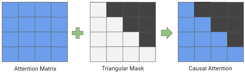
In addition to self-attention, decoder-based transformer models also use casual-attention. This type of attention masks future tokens to prevent the model from “cheating” by using information that is not available at the current time step. It is implemented by masking with the triangular matrix.
attention = attention.masked_fill(self.tril[:T, :T] == 0, float('-inf'))
attention = F.softmax(attention, dim=-1)
Multi-Head Attention
Multi-Head Attention capitalizes on the power of multiple heads to learn and calculate diverse attention patterns. This empowers the model to simultaneously focus on information from various representation subspaces at distinct positions. The following example illustrates how Multi-Head Attention module can be implemented with the causal attention mechanism:
class MultiHeadAttention(nn.Module):
    """ multi head of self-attention """

    def __init__(self, num_heads, head_size):
        super().__init__()
        self.num_heads = num_heads
        self.head_size = head_size

        self.key = nn.Linear(head_size, head_size, bias=False)
        self.query = nn.Linear(head_size, head_size, bias=False)
        self.value = nn.Linear(head_size, head_size, bias=False)
        self.register_buffer('tril', torch.tril(torch.ones(block_size, block_size)))

        self.dropout_wei = nn.Dropout(dropout)
        n_embd= num_heads*head_size
        self.proj = nn.Linear(n_embd, n_embd)
        self.dropout_proj = nn.Dropout(dropout)


    def forward(self, x):
        # Reshape the tensor to B N T H for N heads
        B,T,C = x.shape
        x = rearrange(x, 'B T (N H) -> B N T H', N=self.num_heads)

        k = self.key(x)   # (B,N,T,H)
        q = self.query(x) # (B,N,T,H)

        # compute attention scores \
        wei = torch.einsum("BNTH, BNSH -> BNTS", q,k) * self.head_size**-0.5
        wei = wei.masked_fill(self.tril[:T, :T] == 0, float('-inf'))
        wei = F.softmax(wei, dim=-1)
        wei = self.dropout_wei(wei)
        # perform the weighted aggregation of the values
        v = self.value(x) # (B,N,T,H)
        out = torch.einsum("BNTS, BNSH -> BNTH", wei, v)

        # concat and mix N Heads
        out = rearrange(out, 'B N T H -> B T (N H)')
        out = self.dropout_proj(self.proj(out))
        return out
Transformer Block
The building block of the transformer is crafted by fusing Multi-Head Attention with layer normalization, a non-linear MLP, and residual connections. Within a transformer-based Language Model (LLM), several layers of this foundational transformer block are used to capture intricate contextual relationships and produce cohesive output.
class TransformerBlock(nn.Module):
    """ Transformer block: communication followed by computation """

    def __init__(self, n_embd, n_head):
        # n_embd: embedding dimension, n_head: the number of heads we'd like
        super().__init__()
        head_size = n_embd // n_head
        self.sa = MultiHeadAttention(n_head, head_size)
        self.ffwd = FeedFoward(n_embd)
        self.ln1 = nn.LayerNorm(n_embd)
        self.ln2 = nn.LayerNorm(n_embd)

    def forward(self, x):
        x = x + self.sa(self.ln1(x))
        x = x + self.ffwd(self.ln2(x))
        return x
Implementing and Training mini-GPT model
Basic Bigram Model
Before we dive into the complexities of building a GPT, let’s start with the basics. A bigram model is a simple language model that predicts the next word in a sequence based on the previous word. Here’s an example of a BigramLanguageModel class:
class BigramLanguageModel(nn.Module):
    def __init__(self, vocab_size):
        super().__init__()
        # each token directly maps to the logits for the next token
        self.token_embedding_table = nn.Embedding(vocab_size, vocab_size)

    def forward(self, idx):
        # idx and targets are both (B,T) tensor of integers
        logits = self.token_embedding_table(idx) # (B,T,C)
        return logits

    def generate(self, idx, max_new_tokens):
        # idx is (B, T) array of indices in the current context
        for _ in range(max_new_tokens):
            # get the predictions
            logits, loss = self(idx)
            # focus only on the last time step
            logits = logits[:, -1, :] # becomes (B, C)
            # apply softmax to get probabilities
            probs = F.softmax(logits, dim=-1) # (B, C)
            # sample from the distribution
            idx_next = torch.multinomial(probs, num_samples=1) # (B, 1)
            # append sampled index to the running sequence
            idx = torch.cat((idx, idx_next), dim=1) # (B, T+1)
        return idx
This model can be used to generate text by predicting the next word in a sequence and then feeding that word back into the model to generate the next word. The colab notebook extends the above implementation with loss calculation and depicts simple generative LM training.
While a basic Bigram model can generate coherent text, it has its limitations. For example, it only considers the previous word when making predictions, which can result in repetitive or nonsensical text.
Decoder-based Transformer Model
To overcome the limitations of a basic Bigram model, we can use a decoder-based transformer model. This type of model uses self-attention to consider the entire input sequence when making predictions.
class TransformerModel(nn.Module):
    def __init__(self, vocab_size, n_embd, n_head, max_token_len, n_layer):
        super().__init__()
        # each token directly reads off the logits for the next token from a lookup table
        self.token_embedding_table = nn.Embedding(vocab_size, n_embd)
        self.position_embedding_table = nn.Embedding(max_token_len, n_embd)
        self.blocks = nn.Sequential(*[TransformerBlock(n_embd, n_head=n_head) for _ in range(n_layer)])
        self.ln_f = nn.LayerNorm(n_embd) # final layer norm
        self.lm_head = nn.Linear(n_embd, vocab_size)

    def forward(self, idx, targets=None):
        B, T = idx.shape

        # idx and targets are both (B,T) tensor of integers
        tok_emb = self.token_embedding_table(idx) # (B,T,C)
        pos_emb = self.position_embedding_table(torch.arange(T, device=device)) # (T,C)
        x = tok_emb + pos_emb # (B,T,C)
        x = self.blocks(x) # (B,T,C)
        x = self.ln_f(x) # (B,T,C)
        logits = self.lm_head(x) # (B,T,vocab_size)

        if targets is None:
            loss = None
        else:
            B, T, C = logits.shape
            logits = logits.view(B*T, C)
            targets = targets.view(B*T)
            loss = F.cross_entropy(logits, targets)

        return logits, loss
Optimizations
PreNorm
In PreNorm, the layer normalization is applied before the sublayer (e.g., self-attention or feed-forward) instead of after it, as in the original transformer model (PostNorm). GPT model already utilises PreNorm to provide better training stability.
Weight Tying
This method massively reduces the total number of parameters and improves the performance of language models by tying (sharing) the weights of the embedding and softmax layers. The intuition behind it is that both the embedding layer and the softmax layer learn word representations, such that similar words (in meaning) are represented by vectors that are near each other (in cosine distance). By sharing the weights between these two layers, the model can learn more efficiently and avoid overfitting.
# https://paperswithcode.com/method/weight-tying
self.token_embedding_table.weight = self.lm_head.weight
Flash Attention
The key idea behind Flash Attention is to make the attention algorithm IO-aware, meaning that it takes into account the reads and writes between different levels of GPU memory. Flash Attention uses tiling to load blocks of query, key, and value tensors from GPU high bandwidth memory (HBM) to SRAM (its fast cache). It then computes attention with respect to that block and writes back the output to HBM. By loading in blocks, Flash Attention is able to reduce the number of memory reads/writes between GPU HBM and GPU on-chip SRAM. This results in fewer HBM accesses than standard attention, making Flash Attention 7.5x faster and more memory-efficient.

In Torch 2.0, It can be simply utilised by using torch.nn.functional.scaled_dot_product_attention function. Refer colab section for transformer with flash attention.
Tokenizer
Up until now, we've employed a custom character-level tokenizer, requiring the model to decipher meaning character by character. To simplify this process for the model we can use more abstract units - words and sub-words. Just like, constructing a house is easier using bricks than working with individual grains of cement. However, this approach introduces a new challenge: a notable increase in the count of unique tokens (vocabulary). To address this, we incorporate subword tokenization to strike a balance.
from transformers import GPT2Tokenizer
tokenizer = GPT2Tokenizer.from_pretrained('gpt2')
input_text = "Your input text goes here."
input_ids = tokenizer.encode(input_text)
Typically, I opt for existing tokenization methods, which enable the utilization of pre-trained models. Nonetheless, the beauty of subword tokenization lies in its adaptability to domain-specific text. This is exemplified in the last colab section, where I demonstrate how subword tokenization can be tailored to custom content.
from tokenizers import Tokenizer
from tokenizers.models import BPE
from tokenizers.pre_tokenizers import Whitespace
from tokenizers.trainers import BpeTrainer

tokenizer = Tokenizer(BPE())
tokenizer.pre_tokenizer = Whitespace()
trainer = BpeTrainer(special_tokens=["[UNK]", "[CLS]", "[SEP]", "[PAD]", "[MASK]"])

tokenizer.train_from_iterator(text.split("\n"), trainer=trainer)
tokenizer.get_vocab_size()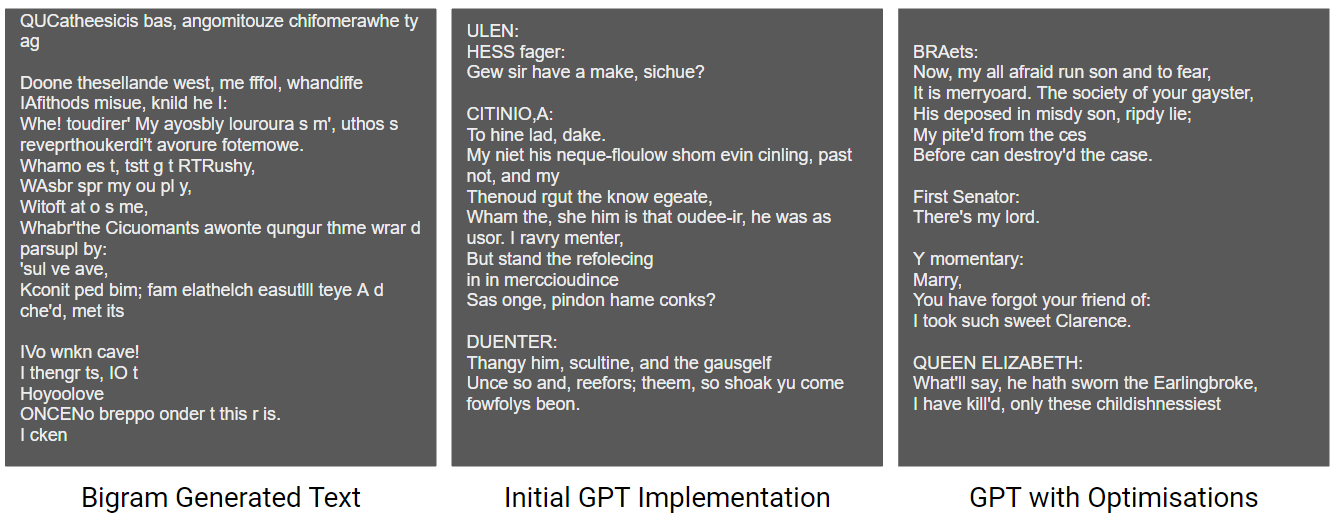
Our generated results significantly improve by integrating these optimizations into our training process for the mini GPT model, even with just 1 million parameters. It's worth noting that state-of-the-art (SOTA) GPT models scale up to sizes exceeding 100 billion parameters, achieving even lower perplexity and more advanced generative capabilities. Nevertheless, despite these scaling differences, the core principles and fundamentals underlying the architecture remain consistent.
What's Next?
Several advancements have been made to improve the capabilities and efficiency of transformer models:
- Integrated Positional embeddings - Fixed, Relative PE (T5), RoPe (llama), AliBi
- Attention optimisations - Efficient attention mechanisms such as Sparse Attention(BIG BIRD), FAVOR+ (Performer), MultiQuery Attention, and Longformer(Sliding Attention).
- Feedforward Network - Optimisations use of CNNs, routing mechanisms
- Training Data - Proper preprocessing and cleaning of training datasets
In our upcoming blog post within this series, our focus will shift towards exploring enhancements related to positional embeddings. Stay tuned and don't hesitate to connect with me on LinkedIn for further discussions.