Understanding the nuances of transformer inference is crucial for optimizing performance and cost. In this blog, we will delve into key concepts such as arithmetic intensity, memory bandwidth, and GPU throughput, going through critical calculations for transformer models like LLaMA 2 on A10 GPUs. We'll explore how to estimate different performance-bound scenarios—whether your model is memory, compute, overhead, or communication-bound—and present strategies for optimizing cost and latency. By the end, you'll have a framework for making informed decisions on how to best utilize your GPU resources for high-throughput transformer inference and a theoretical estimator app comparing costs and performances across different GPUs.

Understanding GPU spec :

Calculate the operations-to-byte (ops:byte) ratio of your GPU from its specifications. For A10 GPU spec:

ops_to_byte_A10
    = compute_bw / memory_bw 
    = 125 TF / 600 GB/S  
    = 208.3 ops / byte

Understanding Transformer Inference Calculations:

• The most computationally expensive part of transformer inference is the attention layer.
• To calculate the arithmetic intensity (operations per byte) of the attention layer, we need to break down the attention equation: $Attention(Q, K, V) = softmax(QK^T/sqrt(d_k))V$
• Let N be the sequence length, d be the dimension of a single attention head, Q, K, and V be matrices of size N by d with fp16/bf16 precision.
• The total compute in floating point operations is approximately: $4(N^2)d + 3N^2$ 
  • Attention Calculation ($A = QK^T$): $2(N^2)d$ FLOPs -  $Q$ and $K$ have dimensions $N \times d$, and their dot product requires $2N^2d$ floating point operations. 
  • Softmax Operation $A = softmax(A)/sqrt(d_k)$:  $3N^2$ FLOPs -  The attention matrix $A$ has size $N^2$. Calculating the exponent for each element requires $N^2$ FLOPs, and the normalization (sum and division across rows) requires an additional $2N^2$ FLOPs. 
  • Output Calculation $O = A.V$: $2(N^2)d$ FLOPs -  $A$ is of size $N \times N$ and $V$ is $N \times d$. The dot product between $A$ and $V$ takes $2N^2d$ FLOPs.
• The total memory movement in bytes is approximately: $8N^2 + 8Nd$ 
  • Attention Calculation $A = QK^T$:  $4Nd + 2N^2$ bytes -  $Q$ and $K$, each of size $N \times d$, require $2Nd$ bytes each in FP16 precision. The resulting attention matrix $A$, of size $N^2$, takes $2N^2$ bytes. 
  • Softmax Operation $A = softmax(A)/sqrt(d_k)$: $4N^2$ bytes -  The input and output of the softmax operation, both of size $N^2$, require $2N^2$ bytes each in FP16. 
  • Output Calculation $O = AV$:  $2N^2 + 4Nd$ bytes -  The attention matrix $A$ of size $N^2$ requires $2N^2$ bytes, and the vectors $V$ and output $O$, both of size $N \times d$, require $2Nd$ bytes each.
• The arithmetic intensity is then calculated as: arithmetic_intensity = $(4(N^2)d + 3N^2) / (8N^2 + 8Nd)$
• For Llama 2 7B, the arithmetic intensity is around 62 operations per byte.

Estimating 4 types of Bound Scenarios:

Compare the ops:byte ratio to the arithmetic intensity of your model.

• Memory Bound: If the arithmetic intensity is lower than the ops:byte ratio, the model is memory bound (limited by memory bandwidth).
• Compute Bound: If the arithmetic intensity is higher than the ops:byte ratio, the model is compute bound (limited by compute resources).
• Overhead Bound: In dynamic languages like PyTorch, the overhead of converting code into GPU execution instructions can sometimes exceed the time spent on execution itself. In such cases, tools like torch.compile or Triton can optimize the execution by reducing overhead.
• Communication Bound: When a significant amount of time is spent on communication between devices, the model is communication-bound. This typically occurs in distributed computing environments.

For Llama 2 7B on an A10 GPU, the model is memory bound during autoregressive sampling (arithmetic intensity of 62 ops/byte < 208.3 ops/byte).

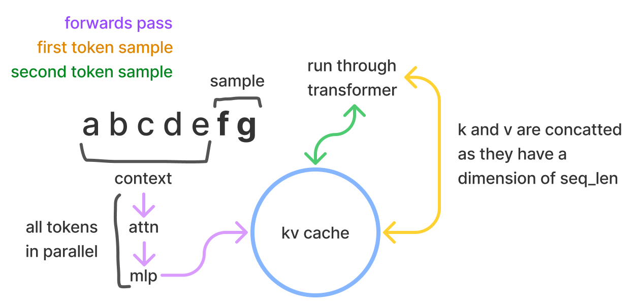
KV cache and batch size estimation

Remaining VRAM = 24 GB - (2 * 7GB) = 10GB # 2 A10 GPU with 12GB VRAM 

kv_cache_size
    = (2 * 2 * n_layers * d_model) bytes/token
    = (4 * 32 * 4096) bytes/token
    = 524288 bytes/token
    ~ 0.00052 GB/token

kv_cache_tokens
    = 10 GB / 0.00052 GB/token
    = 19,230 tokens

batch_size = 19,230/2048 = ~9  => Batch size of 8 can be supported over context len of 2048.

Estimating Cost and Latency:

Prefill time = number of tokens * ( number of parameters / accelerator compute bandwidth)
time/token = total number of bytes moved (the model weights) / accelerator memory bandwidth
Total generation time = prefill time + number of tokens * time/token

For A10, llama 7B models:

prefill_time = 350 * (2 * 7B) FLOP / 125 TFLOP/s = 39 ms
time/token = (2 * 7B) bytes / (600 GB/s) = 23 ms/token
Total Generation Time = 39 ms + 150 tokens * 23 ms/token = 3.49 s

For example, on 2 A100 GPUs with a batch size of 1 for Llama 7B, the estimated cost is $0.066 per 1K tokens, which is higher than GPT-3.5's cost.
Increasing the batch size can reduce the cost but may increase latency.

Model Bandwidth Utilization (MBU):

• MBU measures what percentage of the GPU's memory bandwidth is being utilized during inference.
• It is calculated as: (model_size_in_bytes * tokens_per_second) / GPU_memory_bandwidth
• Higher MBU indicates better utilization of the GPU's memory bandwidth capabilities.
• The above token time estimates are with 100% MBU but in typical experiments, 70% MBU is achieved. These numbers can be scaled to match more real-world scenarios.

Optimizing Performance:

1. Batching: Run forward passes through the model in batches to reuse parts of the model loaded into GPU memory, increasing arithmetic intensity.
   
2. Quantization: Use lower-precision quantization (e.g., INT8, INT4) to reduce the memory bandwidth required for loading model weights.
   
3. Speculative Decoding: Use a smaller "draft" model to generate tokens quickly, then verify them with the larger "verifier" model, reducing the number of times the larger model's weights need to be loaded.
   
4. Tensor Parallelism: Split the model across multiple GPUs to leverage more memory bandwidth and compute resources, improving latency.
   
5. Kernel Optimization and Compilation: Tools like torch.compile can generate highly optimized kernels for operations like matrix multiplications and attention, sometimes outperforming hand-tuned libraries like cuBLAS and FlashAttention.
6. Communication Overhead: Communication overhead between devices, like during model parallelism, can be a significant bottleneck and should be accounted for in performance estimations.

Awesome Resources

A guide to LLM inference and performance

Learn if LLM inference is compute or memory bound to fully utilize GPU power. Get insights on better GPU resource utilization.

BasetenVarun Shenoy

1. GPU specs - Calculating the operations per byte (ops:byte) ratio
2. LLM - Calculating arithmetic intensity
   2.1 Prefill: Prompt processing (processing the input tokens) is compute-bound and relatively inexpensive compared to token generation.
   2.2 Autoregressive sampling: Token generation is memory-bound, as it requires loading the model weights for each generated token, making it more expensive.
3. KV cache and supported batch size estimation.
4. Token Generation Time Estimation
5. Cost Estimations

Transformer Inference Arithmetic | kipply’s blog

kipply’s blog about stuff she does or reads about or observes

kipply's blog

Roofline Paper - understanding performance measurement

Introduction to Holistic Trace Analysis — PyTorch Tutorials 2.3.0+cu121 documentation

Other techniques like Grouped Query Attention, MOE, Paged Attention, Flash Attention, Prefix caching etc improve LLM performance. -> these can be added to corresponding bound scenarios to as improvement examples.

Here is a simple cost estimator with defaults for the Llama 70B model with 8 CB factor (due to Grouped Query Attn) and achieved GPU utilisation (MFU) of 70%. (Colab Notebook Reference)